Every now and then I get a crazy idea. Most of the time I’m smart enough to ignore it, but sometimes, in a moment of insanity, I convince myself the idea is the best one I’ve ever had. Two months ago, that idea was to try and run 5km in under 20 minutes.

Unless you’re an experienced runner, you don’t just put on your running shoes, hop out the door, and run 5km in under 20 minutes. It takes time to train and condition your body to put up with the unfamiliar stress. Since the insanity took over, I’ve been training three times a week, gradually building up speed and stamina. I’m a very long way off, but my time is already down to 25 minutes.

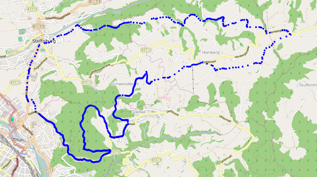
I’ve been using my Garmin Forerunner 210 to record my progress. Like many gadgets it has a built-in GPS receiver, allowing the watch to not only record how long my run is, but also where I run.

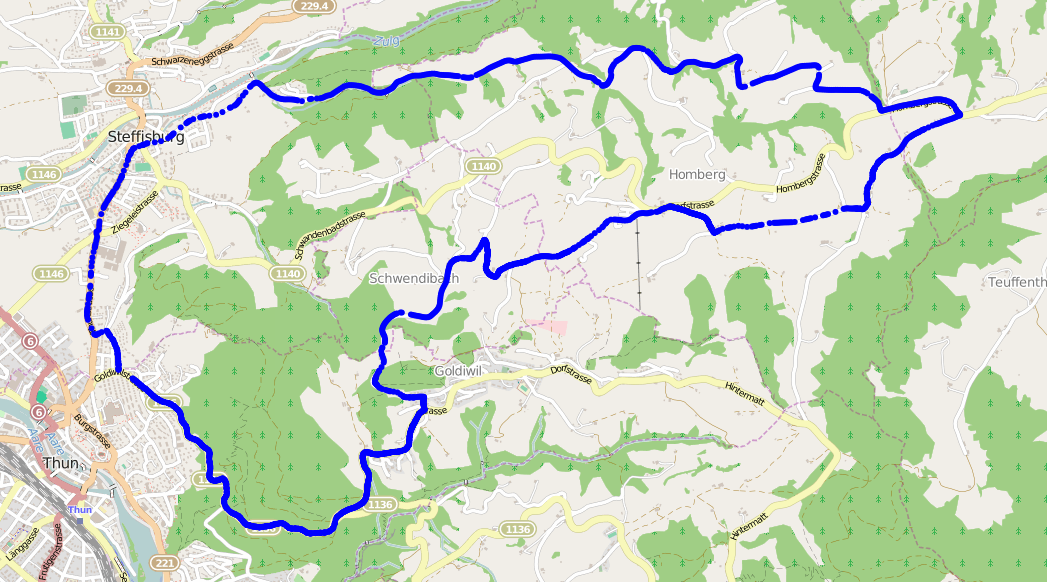
Running the same route every time can be really boring. Almost as boring as reading the longest introduction to a blog post that you’ve ever come across. To keep things interesting, I take slight detours on my routes. The detours also mean I’m less aware that I might be running too slow, which would give me the impulse to give up, find the nearest bus stop, and never think of running again!

Then it happened again. Another crazy idea promptly added to the best-ever pile: can I automatically compare GPS tracks to see where they differ?

Aligning Protein Sequences

Just like when I go running, I’m going to make a slight detour and talk about protein sequences. Don’t worry, it’s related!

Aligning protein sequences is really useful. It allows bioinformaticians to find regions of similarity which may be a consequence of functional, structural, or evolutionary relationships between the sequences.

Sequence 1: TTCCPSIVARSNFNVCRLPGTPEAICATYTGCIIIPGATCPGDYAN
Sequence 2: TCCPSIVARRSNFNVCRLTPEAICATYTGCIIIPGATSPGDYAN

When the above sequences are aligned, gaps are shown to indicate insertions and deletions.

Alignment 1: TTCCPSIVA-RSNFNVCRLPGTPEAICATYTGCIIIPGATCPGDYAN
Alignment 2: -TCCPSIVARRSNFNVCRL--TPEAICATYTGCIIIPGATSPGDYAN

One of the earliest methods for aligning sequences is the Needleman-Wunsch algorithm, published in 1970.

At the heart of the algorithm is the scoring system, which is used to determine how a pair of residues should align. The higher the score for a given combination, the more it is biased in the resulting alignment.

A gap penalty is also applied during alignment. If the gap penalty is greater than the score for aligning two residues, a gap is introduced in the alignment instead.

You can use any scoring system you like, depending on the problem you’re trying to solve. BLOSUM is a similarity matrix commonly used as the scoring system to align protein sequences. It takes into account the likelihood that a residue will mutate into another based on what has already been observed in nature.

Aligning GPS tracks

How many of you skipped the bit about protein sequences? Come on, be honest. It’s okay, I don’t mind, but you might be confused if you don’t read that first.

Hopefully you can already see the connection: instead of aligning residues in protein sequences, we’ll be aligning co-ordinates in GPS tracks. The bits that don’t align, the gaps, will be the sections of the tracks that differ.

But what scoring system and gap penalty should be used?

When we compare tracks by eye, we look at the distance between points. We can use the same metric to score GPS points in the alignment; however, the Needleman-Wunsch algorithm considers higher values a match.

Higher distances mean the points are further apart and therefore non-matching, so we need to use the negative distance as the score, which results in larger distances having smaller values.

The gap penalty works as the cutoff for when the distance between two points is considered large enough that they don’t represent the same location. As the distance is always negative, the gap penalty distance must also be negative.

There is no universal value for this cutoff. It depends on the quality of the data and the context.

If the GPS device is accurate to 5 metres, setting the cutoff to 2 metres will result in a noisy alignment. Likewise, if the tracks being compared are from planes, you might consider them on the same flight path if they are within 200 metres of one another; for tracks of people walking, this distance will be far too large.

So what happens if we use all this information to align two GPS tracks stored in a GPX file and plot them on a map, showing the matched points in blue and the differences in red and orange?

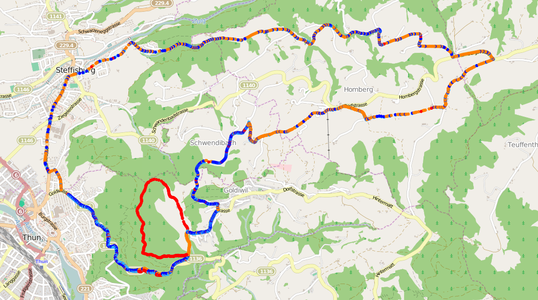
It’s not bad, but also not perfect. It’s found the major detour at the bottom- left of the map (in red), but there are also a lot of incorrect mismatches spread throughout the tracks (in orange). What’s causing this?

The GPS points in the two tracks are not evenly distributed, resulting in points that are far apart being compared when the density in a section of one track differs greatly from the other. If you look at the locations of the orange points in the alignment, they match very closely to the low-density regions in the plot of the first track shown in the introduction.

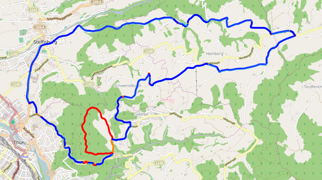
This is fixed by pre-processing the GPX files to distribute GPS points evenly over the track ¹. The closer together the points, the more accurate the result, but the longer the alignment will take.

So how does it look now? Amazing!

Show me the code

There are more examples, along with the code to generate your own alignments, in the jonblack/cmpgpx repository on GitHub. It’s in the public domain, too, so do what you please with it. Yay!